Manual
This manual provides some key concepts important to understand how Spring Model works. For usage examples, with walkthrough instructions are available in tutorial section.
Topics
Method overview
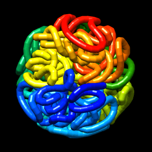
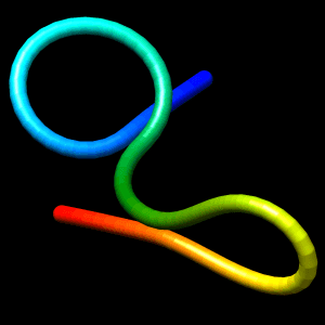
Spring model is a webservice for modelling chromatin domains using direct information about contacts derived from experiments like Hi-C or ChIA-PET. It is employs polymer physics and molecular mechanics using OpenMM library. In SM a polymer is represented as a set of connected beads in 3D space. Their centers are distributed uniformly across the polymer chain i.e. distances between any two consecutive beads are constant and equal in bead diameter. User can choose type of initial structure, and define contacts using two formats of input (direct beads indices, and genomic loci). Then energy of system is minimized and structure folds.
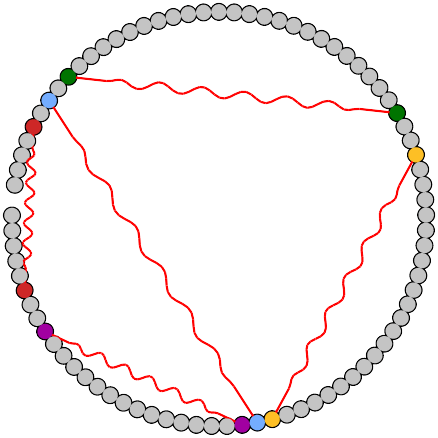 Initial structure
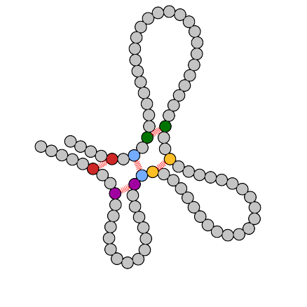 Final structure
Fields description
- Title
- Human readable description, helpful for task identification.
- Initial structure type
Each chromatin model requires an initial structure. Spring model provides several options which may produce different results. The following options are available:
- line
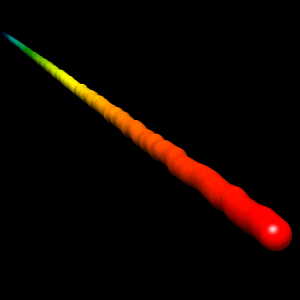
Beads are distributed on an almost straight line. Every bead is slightly distorted in a random direction (maximal distortion length is 0.1σ) to break symmetry.
- circle
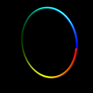
Beads are distributed on a circle. The circle is slightly stretched in z-axis to break symmetry.
- self-avoiding random walk
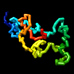
For models that are supposed to start from a random conformation. This kind of random walk consists of spheres that have volume and they cannot overlap.
- pure random walk
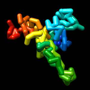
For certain kinds of modelling pure random walk may be a better choice. However, choosing pure random walk and Excluded Volume option may cause the energy of the system to explode due to a high rate of overlaps and cause your simulation to produce artifacts or end up with an error. We recommend to choose this option only with disabled Excluded Volume option. Pure random walks are usually more compacted than self-avoiding random walks.
- baseball
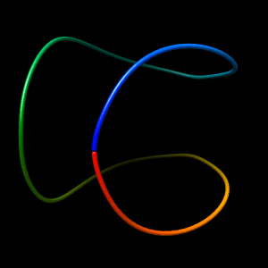
Beads are distributed on a sphere along the curve shaped like a baseball ball seam.
Examples - Click image to download PDB file.
- line
- Stiffness
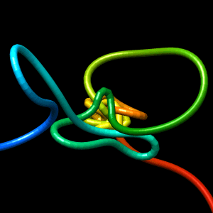
This parameter controls the stiffness of a fiber. Technically it's a harmonic angle force defined between every three consecutive beads across the fiber. It's expressed in units of kJ/mol/rad2. 0 means that there is no stiffness at all. Any other positive value will add an energy term to make the polymer more rod-like than resembling boiled spaghetti. It will cause your loops to look more "inflated", and usually it makes the final structure visually cleaner. High values of this parameter may cause the stiffness to dominate the term associated with interaction energy, and will cause artifacts. For most cases a value of 20 kJ/mol/rad2 is a good first try, and usually it should not exceed 100 kJ/mol/rad2. Remember that excluded volume also implies some extra stiffness to fiber.
Examples - Click image to download PDB file.
- Spherical container
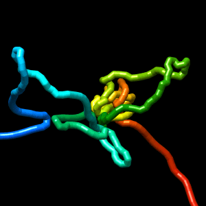
Modelling can be performed in an enclosed sphere-shaped volume. This parameter is the radius of this sphere expressed in σ. Leave it empty if don't want to put any constraints on available volume.
Examples - Click image to download PDB file.
- Refinement
In some cases the energy minimization algorithm can get stuck in a local energy minimum or tend to produce artifacts. In such cases it can be helpful tu run several cycles of short molecular dynamics and energy minimization. The final structure will probably result with lower energy. However, depending on the modeling system it can take much more time. The refinement is performed with following steps:
- Setting up the initial velocities using Boltzmann distribution and temperature 300 K.
- Complete the following 5 times:
- Perform 1000 steps of simulation using Verlet algorithm.
- Perform energy minimization with rough convergence limit of 10 kJ/(nm mol)
- Perform final energy minimization with fine convergence limit of 1 kJ/(nm mol).
Without refinement there will be only one act of energy minimization with coarse 10 kJ/(nm mol) convergence condition.
- Excluded volume
- Volume of the beads. By default it is included, excluding it will cause the beads to become points without volume, allowing the fiber to cross itself freely.
- Number of beads
- Optional. In case of restraints defined in model coordinates this parameter can control the length of the fiber. If it is left empty then the fiber will have the length of the maximum restraint coordinate + 1 bead.
- Restraints
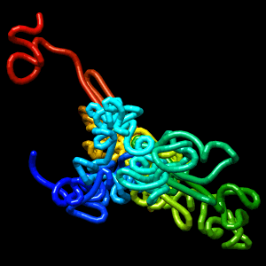
Definition of long-range physical interactions - list of indices of connected beads. Each interaction has to be in a separate line. Coordinates have to be delimited with tab or space. Additionally one may add information about loop type using CTCF directionality notation (i.e. >> >< <> <<) or capital letters S for Stem loop and H for Hairpin loop. Vide example 3 on main site.
Examples - Click image to download PDB file.
- Region
- Optional. In case of modeling based on genomic coordinates this field can control the length of the fiber. If it is left empty then the length of the fiber will be deduced from the maximum coordinate in interactions field and the resolution.
- Resolution
- How much chromatin (number of base pairs) are represented by a single bead. The minimum value is 5 and maximum is limited by the total number of beads which should not exceed 2000.
- Interactions
- Definition of long-range physical interactions. List of interactions in BEDPE file. 7 columns are mandatory and 8th is optional. The middle point of an anchor is taken into account when translating genomic coordinates into bead indices. Value of 7th column is ignored. 8th column can be used to define the loop type in the same way as in the case of restraints.
